Airparif dataset

Disclaimer: this course is adapted from the work Pandas tutorial by Joris Van den Bossche. R users might also want to read Pandas: Comparison with R / R libraries for a smooth start in Pandas.

We start by importing the necessary libraries:

%matplotlib inline
import os
import numpy as np
import calendar
import pandas as pd
import matplotlib.pyplot as plt
import seaborn as sns
from cycler import cycler
import pooch  # download data / avoid re-downloading
from IPython import get_ipython


sns.set_palette("colorblind")
palette = sns.color_palette("twilight", n_colors=12)
pd.options.display.max_rows = 8

This part studies air quality in Paris (Source: Airparif) with pandas.

url = "http://josephsalmon.eu/enseignement/datasets/20080421_20160927-PA13_auto.csv"
path_target = "./20080421_20160927-PA13_auto.csv"
path, fname = os.path.split(path_target)
pooch.retrieve(url, path=path, fname=fname, known_hash=None)

'/home/jsalmon/Documents/Mes_cours/Montpellier/HAX712X/Courses/Pandas/20080421_20160927-PA13_auto.csv'

For instance, you can run in a terminal:

!head -26 ./20080421_20160927-PA13_auto.csv

Alternatively:

from IPython import get_ipython
get_ipython().system('head -26 ./20080421_20160927-PA13_auto.csv')

References:

Working with time series, Python Data Science Handbook by Jake VanderPlas

polution_df = pd.read_csv('20080421_20160927-PA13_auto.csv', sep=';',
                          comment='#',
                          na_values="n/d",
                          converters={'heure': str})

pd.options.display.max_rows = 30
polution_df.head(25)

	date	heure	NO2	O3
0	21/04/2008	1	13.0	74.0
1	21/04/2008	2	11.0	73.0
2	21/04/2008	3	13.0	64.0
3	21/04/2008	4	23.0	46.0
4	21/04/2008	5	47.0	24.0
5	21/04/2008	6	70.0	11.0
6	21/04/2008	7	70.0	17.0
7	21/04/2008	8	76.0	16.0
8	21/04/2008	9	NaN	NaN
9	21/04/2008	10	NaN	NaN
10	21/04/2008	11	NaN	NaN
11	21/04/2008	12	33.0	60.0
12	21/04/2008	13	31.0	61.0
13	21/04/2008	14	37.0	61.0
14	21/04/2008	15	20.0	78.0
15	21/04/2008	16	29.0	71.0
16	21/04/2008	17	30.0	70.0
17	21/04/2008	18	38.0	58.0
18	21/04/2008	19	52.0	40.0
19	21/04/2008	20	56.0	29.0
20	21/04/2008	21	39.0	40.0
21	21/04/2008	22	31.0	42.0
22	21/04/2008	23	29.0	42.0
23	21/04/2008	24	28.0	36.0
24	22/04/2008	1	46.0	16.0

Data preprocessing

# check types
polution_df.dtypes

# check all
polution_df.info()

<class 'pandas.core.frame.DataFrame'>
RangeIndex: 73920 entries, 0 to 73919
Data columns (total 4 columns):
 #   Column  Non-Null Count  Dtype  
---  ------  --------------  -----  
 0   date    73920 non-null  object 
 1   heure   73920 non-null  object 
 2   NO2     71008 non-null  float64
 3   O3      71452 non-null  float64
dtypes: float64(2), object(2)
memory usage: 2.3+ MB

For more info on the nature of Pandas objects, see this discussion on Stackoverflow. Moreover, things are slowly moving from numpy to pyarrow, cf. Pandas user guide

EXERCISE: handling missing values

What is the meaning of “na_values=”n/d” above? Note that an alternative can be obtained with the command polution_df.replace('n/d', np.nan, inplace=True)

Issues with non-conventional hours/day format

Start by changing to integer type (e.g., int8):

polution_df['heure'] = polution_df['heure'].astype(np.int8)
polution_df['heure']

0         1
1         2
2         3
3         4
4         5
         ..
73915    20
73916    21
73917    22
73918    23
73919    24
Name: heure, Length: 73920, dtype: int8

No data is from 1 to 24… not conventional so let’s make it from 0 to 23

polution_df['heure'] = polution_df['heure'] - 1
polution_df['heure']

0         0
1         1
2         2
3         3
4         4
         ..
73915    19
73916    20
73917    21
73918    22
73919    23
Name: heure, Length: 73920, dtype: int8

and back to strings:

polution_df['heure'] = polution_df['heure'].astype('str')
polution_df['heure']

0         0
1         1
2         2
3         3
4         4
         ..
73915    19
73916    20
73917    21
73918    22
73919    23
Name: heure, Length: 73920, dtype: object

Time processing

Note that we have used the following conventions:

d = day
m=month
Y=year
H=hour
M=minutes

time_improved = pd.to_datetime(polution_df['date'] +
                               ' ' + polution_df['heure'] + ':00',
                               format='%d/%m/%Y %H:%M')

time_improved

0       2008-04-21 00:00:00
1       2008-04-21 01:00:00
2       2008-04-21 02:00:00
3       2008-04-21 03:00:00
4       2008-04-21 04:00:00
                ...        
73915   2016-09-27 19:00:00
73916   2016-09-27 20:00:00
73917   2016-09-27 21:00:00
73918   2016-09-27 22:00:00
73919   2016-09-27 23:00:00
Length: 73920, dtype: datetime64[ns]

polution_df['date'] + ' ' + polution_df['heure'] + ':00'

0         21/04/2008 0:00
1         21/04/2008 1:00
2         21/04/2008 2:00
3         21/04/2008 3:00
4         21/04/2008 4:00
               ...       
73915    27/09/2016 19:00
73916    27/09/2016 20:00
73917    27/09/2016 21:00
73918    27/09/2016 22:00
73919    27/09/2016 23:00
Length: 73920, dtype: object

Create correct timing format in the dataframe

polution_df['DateTime'] = time_improved
 # remove useless columns:
del polution_df['heure']
del polution_df['date']
polution_df

	NO2	O3	DateTime
0	13.0	74.0	2008-04-21 00:00:00
1	11.0	73.0	2008-04-21 01:00:00
2	13.0	64.0	2008-04-21 02:00:00
3	23.0	46.0	2008-04-21 03:00:00
4	47.0	24.0	2008-04-21 04:00:00
...	...	...	...
73915	55.0	31.0	2016-09-27 19:00:00
73916	85.0	5.0	2016-09-27 20:00:00
73917	75.0	9.0	2016-09-27 21:00:00
73918	64.0	15.0	2016-09-27 22:00:00
73919	57.0	14.0	2016-09-27 23:00:00

73920 rows × 3 columns

Visualize the data set now that the time is well formatted:

polution_ts = polution_df.set_index(['DateTime'])
polution_ts = polution_ts.sort_index(ascending=True)
polution_ts.head(12)

	NO2	O3
DateTime
2008-04-21 00:00:00	13.0	74.0
2008-04-21 01:00:00	11.0	73.0
2008-04-21 02:00:00	13.0	64.0
2008-04-21 03:00:00	23.0	46.0
2008-04-21 04:00:00	47.0	24.0
2008-04-21 05:00:00	70.0	11.0
2008-04-21 06:00:00	70.0	17.0
2008-04-21 07:00:00	76.0	16.0
2008-04-21 08:00:00	NaN	NaN
2008-04-21 09:00:00	NaN	NaN
2008-04-21 10:00:00	NaN	NaN
2008-04-21 11:00:00	33.0	60.0

polution_ts.describe()

	NO2	O3
count	71008.000000	71452.000000
mean	34.453414	39.610046
std	20.380702	28.837333
min	1.000000	0.000000
25%	19.000000	16.000000
50%	30.000000	38.000000
75%	46.000000	58.000000
max	167.000000	211.000000

fig, axes = plt.subplots(2, 1, figsize=(6, 6), sharex=True)

axes[0].plot(polution_ts['O3'])
axes[0].set_title("Ozone polution: daily average in Paris")
axes[0].set_ylabel("Concentration (µg/m³)")

axes[1].plot(polution_ts['NO2'])
axes[1].set_title("Nitrogen polution: daily average in Paris")
axes[1].set_ylabel("Concentration (µg/m³)")
plt.show()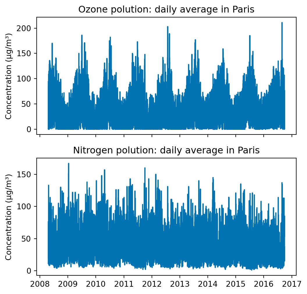

fig, axes = plt.subplots(2, 1, figsize=(10, 5), sharex=True)

axes[0].plot(polution_ts['O3'].resample('d').max(), '--')
axes[0].plot(polution_ts['O3'].resample('d').min(),'-.')

axes[0].set_title("Ozone polution: daily average in Paris")
axes[0].set_ylabel("Concentration (µg/m³)")

axes[1].plot(polution_ts['NO2'].resample('d').max(),  '--')
axes[1].plot(polution_ts['NO2'].resample('d').min(),  '-.')

axes[1].set_title("Nitrogen polution: daily average in Paris")
axes[1].set_ylabel("Concentration (µg/m³)")

plt.show()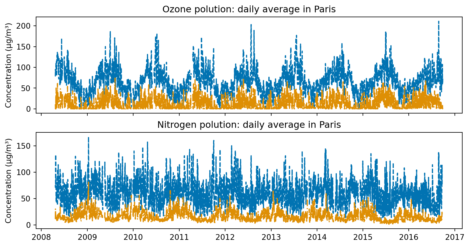

Source : https://www.tutorialspoint.com/python/time_strptime.htm

EXERCISE: extreme values per day

Provide the same plots as before, but with daily best and worst on the same figures (and use different colors and/or styles)

Q: Is the pollution getting better over the years or not?

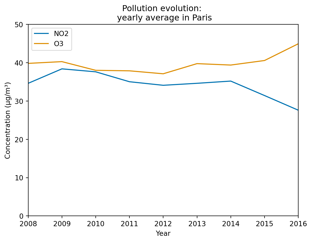
fig, ax = plt.subplots(1, 1)
polution_ts['2008':].resample('Y').mean().plot(ax=ax)
# Sample by year (A pour Annual) or Y for Year
plt.ylim(0, 50)
plt.title("Pollution evolution: \n yearly average in Paris")
plt.ylabel("Concentration (µg/m³)")
plt.xlabel("Year")
plt.show()

Loading colors:

sns.set_palette("GnBu_d", n_colors=7)
polution_ts['weekday'] = polution_ts.index.weekday  # Monday=0, Sunday=6
polution_ts['weekend'] = polution_ts['weekday'].isin([5, 6])

polution_week_no2 = polution_ts.groupby(['weekday', polution_ts.index.hour])[
    'NO2'].mean().unstack(level=0)
polution_week_03 = polution_ts.groupby(['weekday', polution_ts.index.hour])[
    'O3'].mean().unstack(level=0)
plt.show()

fig, axes = plt.subplots(2, 1, figsize=(7, 7), sharex=True)

polution_week_no2.plot(ax=axes[0])
axes[0].set_ylabel("Concentration (µg/m³)")
axes[0].set_xlabel("Intraday evolution")
axes[0].set_title(
    "Daily NO2 concentration: weekend effect?")
axes[0].set_xticks(np.arange(0, 24))
axes[0].set_xticklabels(np.arange(0, 24), rotation=45)
axes[0].set_ylim(0, 60)

polution_week_03.plot(ax=axes[1])
axes[1].set_ylabel("Concentration (µg/m³)")
axes[1].set_xlabel("Intraday evolution")
axes[1].set_title("Daily O3 concentration: weekend effect?")
axes[1].set_xticks(np.arange(0, 24))
axes[1].set_xticklabels(np.arange(0, 24), rotation=45)
axes[1].set_ylim(0, 70)
axes[0].legend().set_visible(False)
# ax.legend()
axes[1].legend(labels=[day for day in calendar.day_name], loc='lower left', bbox_to_anchor=(1, 0.1))

plt.tight_layout()
plt.show()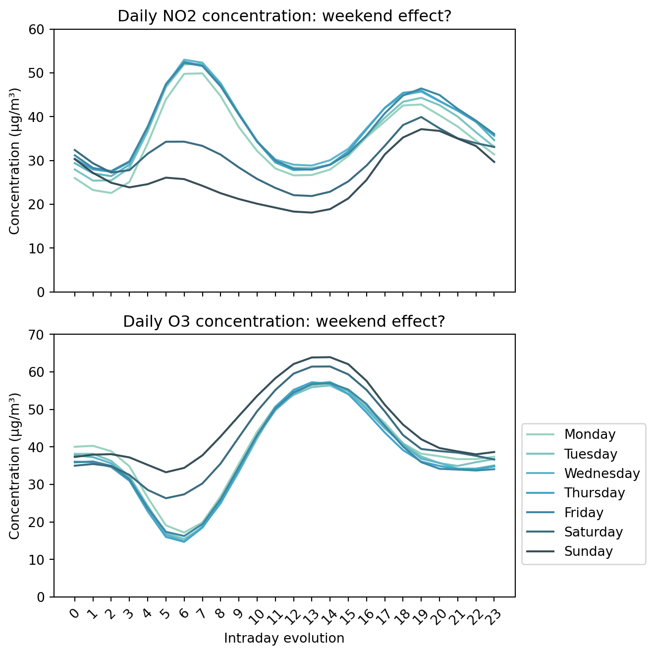

polution_ts['month'] = polution_ts.index.month  # Janvier=0, .... Decembre=11
polution_ts['month'] = polution_ts['month'].apply(lambda x:
                                                  calendar.month_abbr[x])
polution_ts.head()

	NO2	O3	weekday	weekend	month
DateTime
2008-04-21 00:00:00	13.0	74.0	0	False	Apr
2008-04-21 01:00:00	11.0	73.0	0	False	Apr
2008-04-21 02:00:00	13.0	64.0	0	False	Apr
2008-04-21 03:00:00	23.0	46.0	0	False	Apr
2008-04-21 04:00:00	47.0	24.0	0	False	Apr

polution_month_no2 = polution_ts.groupby(['month', polution_ts.index.hour])[
    'NO2'].mean().unstack(level=0)
polution_month_03 = polution_ts.groupby(['month', polution_ts.index.hour])[
    'O3'].mean().unstack(level=0)

fig, axes = plt.subplots(2, 1, figsize=(7, 7), sharex=True)

axes[0].set_prop_cycle(
    (
        cycler(color=palette) + cycler(ms=[4] * 12)
        + cycler(marker=["o", "^", "s", "p"] * 3)
        + cycler(linestyle=["-", "--", ":", "-."] * 3)
    )
)
polution_month_no2.plot(ax=axes[0])
axes[0].set_ylabel("Concentration (µg/m³)")
axes[0].set_xlabel("Hour of the day")
axes[0].set_title(
    "Daily profile per month (NO2)?")
axes[0].set_xticks(np.arange(0, 24))
axes[0].set_xticklabels(np.arange(0, 24), rotation=45)
axes[0].set_ylim(0, 90)

axes[1].set_prop_cycle(
    (
        cycler(color=palette) + cycler(ms=[4] * 12)
        + cycler(marker=["o", "^", "s", "p"] * 3)
        + cycler(linestyle=["-", "--", ":", "-."] * 3)
    )
)
polution_month_03.plot(ax=axes[1])
axes[1].set_ylabel("Concentration (µg/m³)")
axes[1].set_xlabel("Hour of the day")
axes[1].set_title("Daily profile per month (O3): weekend effect?")
axes[1].set_xticks(np.arange(0, 24))
axes[1].set_xticklabels(np.arange(0, 24), rotation=45)
axes[1].set_ylim(0, 90)

axes[0].legend().set_visible(False)
# ax.legend()
axes[1].legend(labels=calendar.month_name[1:], loc='lower left',
               bbox_to_anchor=(1, 0.1))
plt.tight_layout()
plt.show()

References:

Other interactive tools for data visualization: Altair, Bokeh. See comparisons by Aarron Geller: link
An interesting tutorial: Altair introduction
Introduction on geopandas
Notebook on French departememen/womennts issues
Choropleth Maps in practice with Plotly and Python by Thibaud Lamothe
European data on France geography