Titanic dataset

Disclaimer: this course is adapted from the work Pandas tutorial by Joris Van den Bossche. R users might also want to read Pandas: Comparison with R / R libraries for a smooth start in Pandas.

We start by importing the necessary libraries:

%matplotlib inline
import os
import numpy as np
import calendar
import pandas as pd
import matplotlib.pyplot as plt
import seaborn as sns
from cycler import cycler
import pooch  # download data / avoid re-downloading
from IPython import get_ipython


sns.set_palette("colorblind")
palette = sns.color_palette("twilight", n_colors=12)
pd.options.display.max_rows = 8

Data preparation

Automatic data download

First, it is important to download automatically remote files for reproducibility (and avoid typing names manually). Let us apply this to the Titanic dataset:

url = "http://josephsalmon.eu/enseignement/datasets/titanic.csv"
path_target = "./titanic.csv"
path, fname = os.path.split(path_target)
pooch.retrieve(url, path=path, fname=fname, known_hash=None)  # if needed `pip install pooch`

'/home/jsalmon/Documents/Mes_cours/Montpellier/HAX712X/Courses/Pandas/titanic.csv'

Reading the file as a pandas dataframe with read_csv:

df_titanic_raw = pd.read_csv("titanic.csv")

Visualize the end of the dataset:

df_titanic_raw.tail(n=3)

	PassengerId	Survived	Pclass	Name	Sex	Age	SibSp	Parch	Ticket	Fare	Cabin	Embarked
888	889	0	3	Johnston, Miss. Catherine Helen "Carrie"	female	NaN	1	2	W./C. 6607	23.45	NaN	S
889	890	1	1	Behr, Mr. Karl Howell	male	26.0	0	0	111369	30.00	C148	C
890	891	0	3	Dooley, Mr. Patrick	male	32.0	0	0	370376	7.75	NaN	Q

Visualize the beginning of the dataset:

df_titanic_raw.head(n=5)

	PassengerId	Survived	Pclass	Name	Sex	Age	SibSp	Parch	Ticket	Fare	Cabin	Embarked
0	1	0	3	Braund, Mr. Owen Harris	male	22.0	1	0	A/5 21171	7.2500	NaN	S
1	2	1	1	Cumings, Mrs. John Bradley (Florence Briggs Th...	female	38.0	1	0	PC 17599	71.2833	C85	C
2	3	1	3	Heikkinen, Miss. Laina	female	26.0	0	0	STON/O2. 3101282	7.9250	NaN	S
3	4	1	1	Futrelle, Mrs. Jacques Heath (Lily May Peel)	female	35.0	1	0	113803	53.1000	C123	S
4	5	0	3	Allen, Mr. William Henry	male	35.0	0	0	373450	8.0500	NaN	S

Missing values

It is common to encounter features/covariates with missing values. In pandas they were mostly handled as np.nan (not a number) in the past. With versions >=1.0 missing values are now treated as NA (Not Available), in a similar way as in R; see the Pandas documentation on missing data for standard behavior and details.

Note that the main difference between pd.NA and np.nan is that pd.NA propagates even for comparisons:

pd.NA == 1

<NA>

whereas

np.nan == 1

False

Testing the presence of missing values

print(pd.isna(pd.NA), pd.isna(np.nan))

True True

The simplest strategy (when you can / when you have enough samples) consists of removing all nans/NAs, and can be performed with dropna:

df_titanic = df_titanic_raw.dropna()
df_titanic.tail(3)

	PassengerId	Survived	Pclass	Name	Sex	Age	SibSp	Parch	Ticket	Fare	Cabin	Embarked
879	880	1	1	Potter, Mrs. Thomas Jr (Lily Alexenia Wilson)	female	56.0	0	1	11767	83.1583	C50	C
887	888	1	1	Graham, Miss. Margaret Edith	female	19.0	0	0	112053	30.0000	B42	S
889	890	1	1	Behr, Mr. Karl Howell	male	26.0	0	0	111369	30.0000	C148	C

You can see for instance the passenger with PassengerId 888 has been removed by the dropna call.

# Useful info on the dataset (especially missing values!)
df_titanic.info()

<class 'pandas.core.frame.DataFrame'>
Index: 183 entries, 1 to 889
Data columns (total 12 columns):
 #   Column       Non-Null Count  Dtype  
---  ------       --------------  -----  
 0   PassengerId  183 non-null    int64  
 1   Survived     183 non-null    int64  
 2   Pclass       183 non-null    int64  
 3   Name         183 non-null    object 
 4   Sex          183 non-null    object 
 5   Age          183 non-null    float64
 6   SibSp        183 non-null    int64  
 7   Parch        183 non-null    int64  
 8   Ticket       183 non-null    object 
 9   Fare         183 non-null    float64
 10  Cabin        183 non-null    object 
 11  Embarked     183 non-null    object 
dtypes: float64(2), int64(5), object(5)
memory usage: 18.6+ KB

# Check that the `Cabin` information is mostly missing; the same holds for `Age`
df_titanic_raw.info()

<class 'pandas.core.frame.DataFrame'>
RangeIndex: 891 entries, 0 to 890
Data columns (total 12 columns):
 #   Column       Non-Null Count  Dtype  
---  ------       --------------  -----  
 0   PassengerId  891 non-null    int64  
 1   Survived     891 non-null    int64  
 2   Pclass       891 non-null    int64  
 3   Name         891 non-null    object 
 4   Sex          891 non-null    object 
 5   Age          714 non-null    float64
 6   SibSp        891 non-null    int64  
 7   Parch        891 non-null    int64  
 8   Ticket       891 non-null    object 
 9   Fare         891 non-null    float64
 10  Cabin        204 non-null    object 
 11  Embarked     889 non-null    object 
dtypes: float64(2), int64(5), object(5)
memory usage: 83.7+ KB

Other strategies are possible to handle missing values but they are out of scope for this preliminary course on pandas, see the documentation for more details.

Data description

Details of the dataset are given here

• Survived: Survival 0 = No, 1 = Yes
• Pclass: Ticket class 1 = 1st, 2 = 2nd, 3 = 3rd
• Sex: Sex male/female
• Age: Age in years
• Sibsp: # of siblings/spouses aboard the Titanic
• Parch: # of parents/children aboard the Titanic
• Ticket: Ticket number
• Fare: Passenger fare
• Cabin: Cabin number
• Embarked: Port of Embarkation C = Cherbourg, Q = Queenstown, S = Southampton
• Name: Name of the passenger
• PassengerId: Number to identify passenger

Note

For those interested, an extended version of the dataset is available here https://biostat.app.vumc.org/wiki/Main/DataSets.

Simple descriptive statistics can be obtained using the describe method:

df_titanic.describe()

	PassengerId	Survived	Pclass	Age	SibSp	Parch	Fare
count	183.000000	183.000000	183.000000	183.000000	183.000000	183.000000	183.000000
mean	455.366120	0.672131	1.191257	35.674426	0.464481	0.475410	78.682469
std	247.052476	0.470725	0.515187	15.643866	0.644159	0.754617	76.347843
min	2.000000	0.000000	1.000000	0.920000	0.000000	0.000000	0.000000
25%	263.500000	0.000000	1.000000	24.000000	0.000000	0.000000	29.700000
50%	457.000000	1.000000	1.000000	36.000000	0.000000	0.000000	57.000000
75%	676.000000	1.000000	1.000000	47.500000	1.000000	1.000000	90.000000
max	890.000000	1.000000	3.000000	80.000000	3.000000	4.000000	512.329200

Visualization

• Histograms: usually has one parameter controlling the number of bins (please avoid… often useless, when many samples are available)

fig, ax = plt.subplots(1, 1, figsize=(5, 3))
ax.hist(df_titanic['Age'], density=True, bins=25)
plt.xlabel('Age')
plt.ylabel('Proportion')
plt.title("Passager age histogram")
plt.show()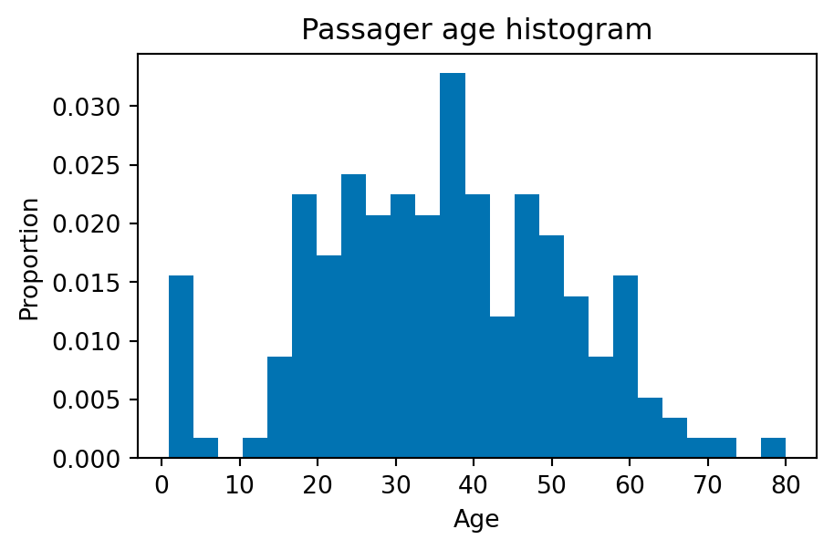

• Kernel Density Estimate (KDE): usually has one parameter (the bandwidth) controlling the smoothing level.

fig, ax = plt.subplots(1, 1, figsize=(5, 3))
sns.kdeplot(
    df_titanic["Age"], ax=ax, fill=True, cut=0, bw_adjust=0.1
)
plt.xlabel("Proportion")
plt.ylabel("Age")
plt.title("Passager age kernel density estimate")
plt.tight_layout()
plt.show()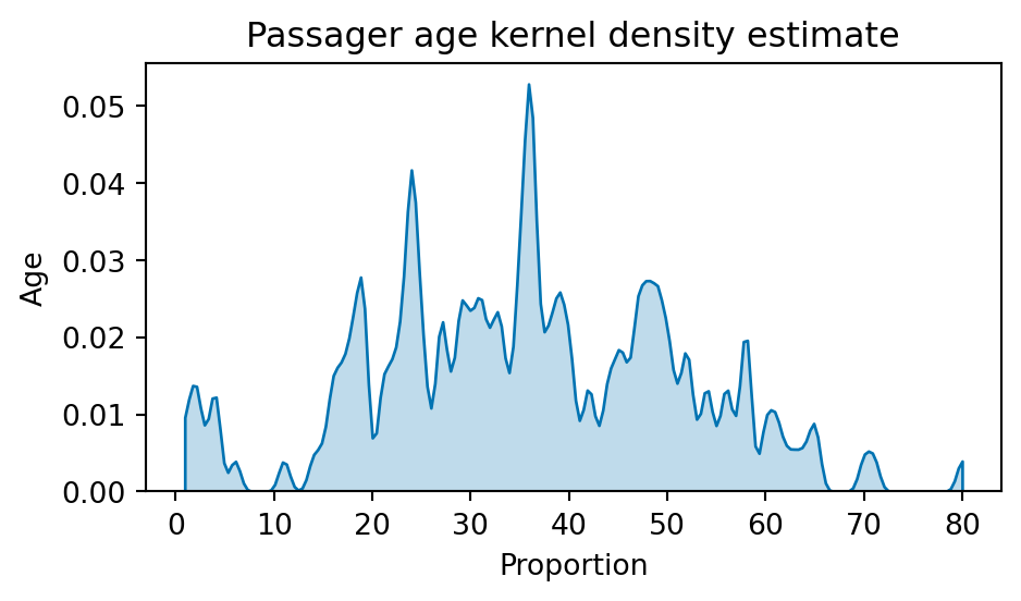

Note

The bandwidth parameter (here encoded as bw_adjust) controls the smoothing level. It is a common parameter in kernel smoothing, investigated thoroughly in the non-parametric statistics literature.

• Swarmplot:

fig, ax = plt.subplots(1, 1, figsize=(6, 5))
sns.swarmplot(
    data=df_titanic_raw,
    ax=ax,
    x="Sex",
    y="Age",
    hue="Survived",
    palette={0: "r", 1: "k"},
    order=["female", "male"],
)
plt.title("Passager age by gender/survival")
plt.legend(labels=["Survived", "Died"], loc="upper left")
plt.tight_layout()
plt.show()

EXERCISE density over histogram

Plot the density estimate over the histogram

Interactivity

Interactive interaction with codes and output is nowadays getting easier and easier (see also Shiny app in R-software). In Python, one can use plotly, or widgets and the interact package for this purpose. We are going to visualize that on the simple KDE and histogram examples.

import plotly.graph_objects as go
import numpy as np
from scipy import stats

# Create figure
fig = go.FigureWidget()

# Add traces, one for each slider step
bws = np.arange(0.01, 0.51, 0.01)
xx = np.arange(0, 100, 0.5)
for step in bws:
    kernel = stats.gaussian_kde(df_titanic["Age"], bw_method=step)
    yy = kernel(xx)
    fig.add_trace(
        go.Scatter(
            visible=False,
            fill="tozeroy",
            fillcolor="rgba(67, 67, 67, 0.5)",
            line=dict(color="black", width=2),
            name=f"Bw = {step:.2f}",
            x=xx,
            y=yy,
        )
    )

# Make 10th trace visible
fig.data[10].visible = True

# Create and add slider
steps = []
for i in range(len(fig.data)):
    step = dict(
        method="update",
        args=[{"visible": [False] * len(fig.data)}],
        label=f"{bws[i]:.2f}",
    )
    step["args"][0]["visible"][i] = True  # Toggle i'th trace to "visible"
    steps.append(step)
sliders = [
    dict(
        active=10,
        currentvalue={"prefix": "Bandwidth = "},
        pad={"t": 50},
        steps=steps,
    )
]

fig.update_layout(
    sliders=sliders,
    template="simple_white",
    title=f"Impact of the bandwidth on the KDE",
    showlegend=False,
    xaxis_title="Age"
)

fig.show()

import plotly.graph_objects as go
import numpy as np
from scipy import stats

# Create figure
fig = go.FigureWidget()

# Add traces, one for each slider step
bws = np.arange(0.01, 5.51, 0.3)
xx = np.arange(0, 100, 0.5)

for step in bws:
    fig.add_trace(
        go.Histogram(
            x=df_titanic["Age"],
            xbins=dict(  # bins used for histogram
                start=xx.min(),
                end=xx.max(),
                size=step,
            ),
            histnorm="probability density",
            autobinx=False,
            visible=False,
            marker_color="rgba(67, 67, 67, 0.5)",
            name=f"Bandwidth = {step:.2f}",
        )
    )

# Make 10th trace visible
fig.data[10].visible = True
# Create and add slider
steps = []
for i in range(len(fig.data)):
    step = dict(
        method="update",
        args=[{"visible": [False] * len(fig.data)}],
        label=f"{bws[i]:.2f}",
    )
    step["args"][0]["visible"][i] = True  # Toggle i'th trace to "visible"
    steps.append(step)
sliders = [
    dict(
        active=10,
        currentvalue={"prefix": "Bandwidth = "},
        pad={"t": 50},
        steps=steps,
    )
]

fig.update_layout(
    sliders=sliders,
    template="simple_white",
    title=f"Impact of the bandwidth on histograms",
    showlegend=False,
    xaxis_title="Age"
)

fig.show()

IPython widgets (in Jupyter notebooks)

import ipywidgets as widgets
from ipywidgets import interact, fixed

def hist_explore(
    dataset=df_titanic,
    variable=df_titanic.columns,
    n_bins=24,
    alpha=0.25,
    density=False,
):
    fig, ax = plt.subplots(1, 1, figsize=(5, 5))
    ax.hist(dataset[variable], density=density, bins=n_bins, alpha=alpha)
    plt.ylabel("Density level")
    plt.title(f"Dataset {dataset.attrs['name']}:\n Histogram for passengers' age")
    plt.tight_layout()
    plt.show()


interact(
    hist_explore,
    dataset=fixed(df_titanic),
    n_bins=(1, 50, 1),
    alpha=(0, 1, 0.1),
    density=False,
)

def kde_explore(dataset=df_titanic, variable=df_titanic.columns, bw=5):
    fig, ax = plt.subplots(1, 1, figsize=(5, 5))
    sns.kdeplot(dataset[variable], bw_adjust=bw, fill=True, cut=0, ax=ax)
    plt.ylabel("Density level")
    plt.title(f"Dataset:\n KDE for passengers'  {variable}")
    plt.tight_layout()
    plt.show()

interact(kde_explore, dataset=fixed(df_titanic), bw=(0.001, 2, 0.01))

Data wrangling

groupby function

Here is an example of the using the groupby function:

df_titanic.groupby(['Sex'])[['Survived', 'Age', 'Fare', 'Pclass']].mean()

	Survived	Age	Fare	Pclass
Sex
female	0.931818	32.676136	89.000900	1.215909
male	0.431579	38.451789	69.124343	1.168421

You can answer other similar questions, such as “how does the survival rate change w.r.t. to sex”?

df_titanic_raw.groupby('Sex')[['Survived']].aggregate(lambda x: x.mean())

	Survived
Sex
female	0.742038
male	0.188908

How does the survival rate change w.r.t. the class?

df_titanic.columns

Index(['PassengerId', 'Survived', 'Pclass', 'Name', 'Sex', 'Age', 'SibSp',
       'Parch', 'Ticket', 'Fare', 'Cabin', 'Embarked'],
      dtype='object')

fig, ax = plt.subplots(1, 1, figsize=(5, 5))

df_titanic.groupby('Pclass')['Survived'].aggregate(lambda x:
                                                   x.mean()).plot(ax=ax,kind='bar')
plt.xlabel('Classes')
plt.ylabel('Survival rate')
plt.title('Survival rate per classs')
plt.show()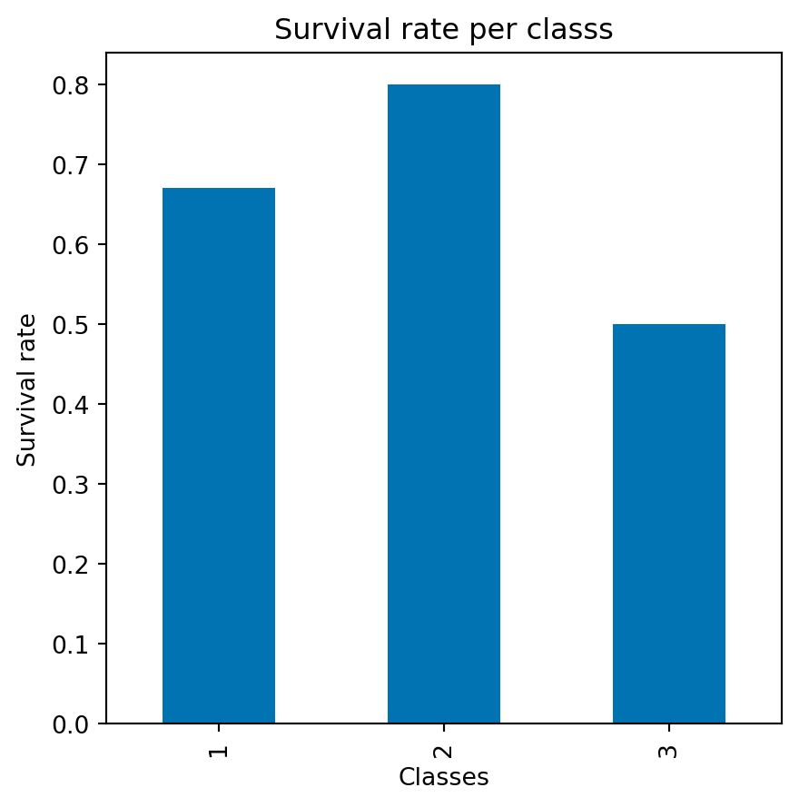

EXERCISE median by class

Perform a similar analysis with the median for the price per class in pounds.

catplot: a visual groupby

ax=sns.catplot(
    x="Pclass",
    y="Age",
    hue="Sex",
    palette={'female': 'red', 'male': 'b'},
    data=df_titanic_raw,
    jitter = '0.2',
    s=8,
)
plt.title("Sex repartition per class on the Titanic")
sns.move_legend(ax, "upper left", bbox_to_anchor=(0.8, 0.8))
plt.show()

ax=sns.catplot(
    x="Pclass",
    y="Age",
    hue="Sex",
    palette={'female': 'red', 'male': 'b'},
    alpha=0.8,
    data=df_titanic_raw,
    kind='swarm',
    s=11,
)
plt.title("Sex repartition per class on the Titanic")
sns.move_legend(ax, "upper left", bbox_to_anchor=(0.8, 0.8))
plt.show()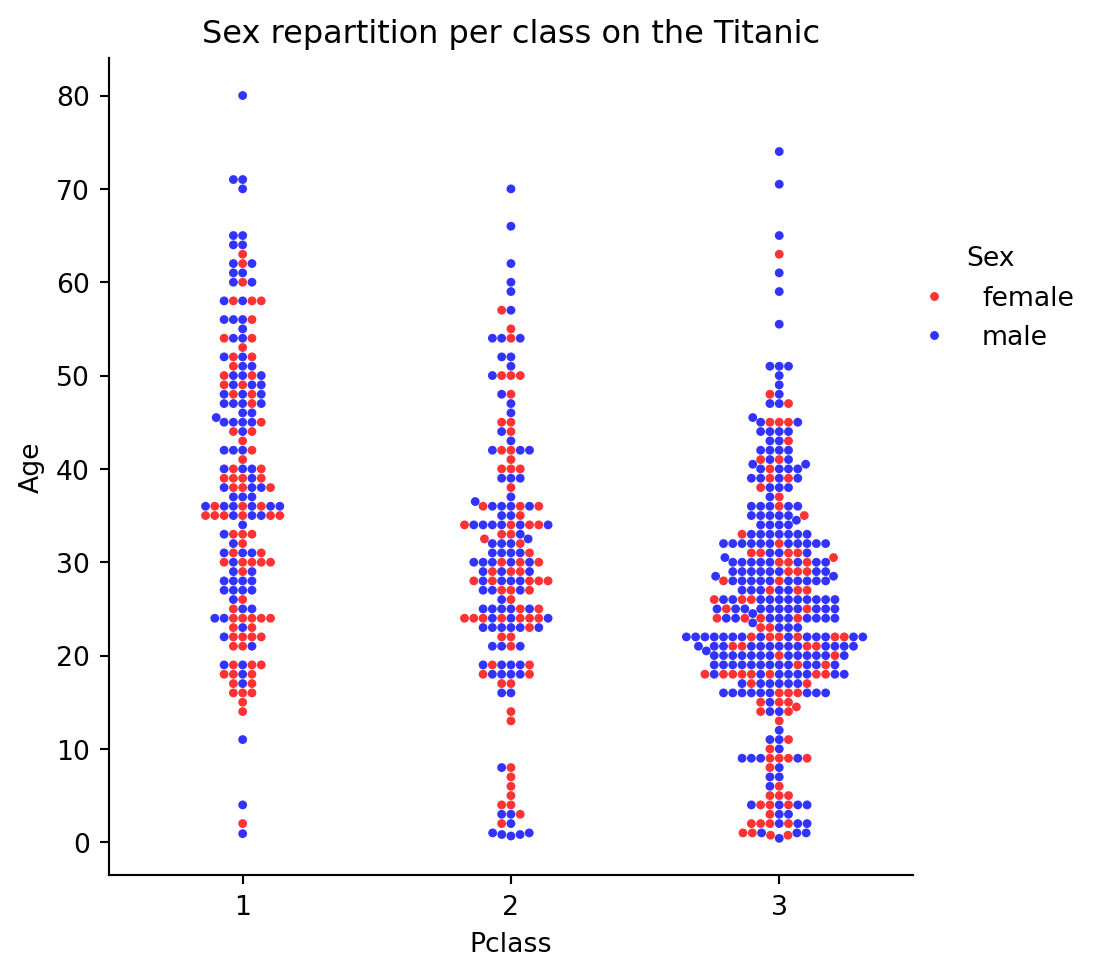

ax=sns.catplot(
    x="Sex",
    y="Age",
    hue="Sex",
    palette={'female': 'red', 'male': 'b'},
    col='Pclass',
    alpha=0.8,
    data=df_titanic_raw,
    kind='swarm',
    s=6,
    height=5,
    aspect=0.49,
)
plt.suptitle("Sex repartition per class on Titanic")
plt.tight_layout()
plt.show()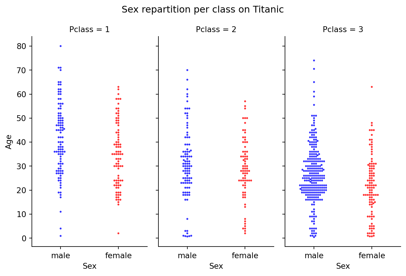

ax=sns.catplot(x='Pclass',
            y='Age',
            hue="Sex",
            palette={'female': 'red', 'male': 'b'},
            data=df_titanic_raw,
            kind="violin",
            alpha=0.8,
)
plt.title("Sex repartition per class on the Titanic")
sns.move_legend(ax, "upper left", bbox_to_anchor=(0.8, 0.8))
plt.show()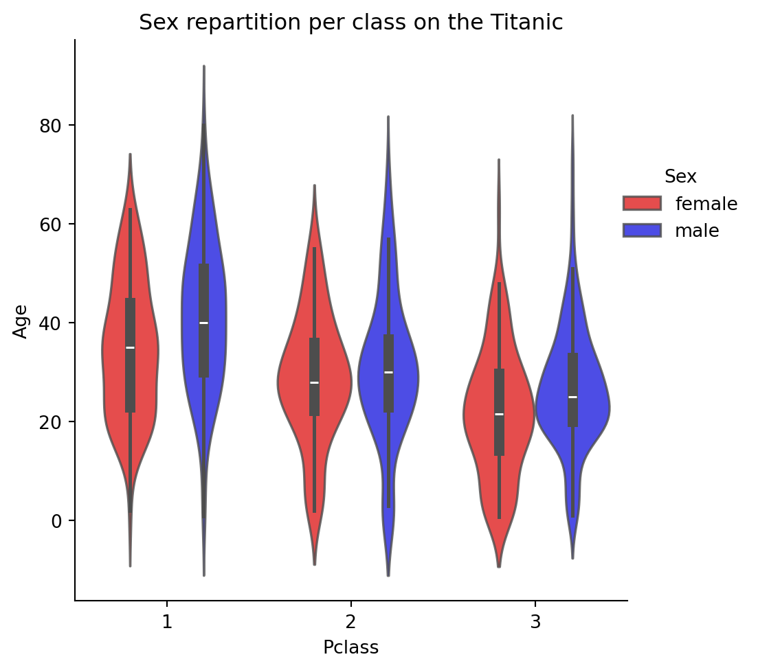

Beware: there is a large difference in sex ratio by class. You can use groups to get the counts illustrating this:

Raw sex repartition per class:

df_titanic_raw.groupby(['Sex', 'Pclass'])[['Sex']].count()

		Sex
Sex	Pclass
female	1	94
	2	76
	3	144
male	1	122
	2	108
	3	347

Raw sex ratio:

df_titanic.groupby(['Sex', 'Pclass'])[['Sex']].count()

		Sex
Sex	Pclass
female	1	74
	2	9
	3	5
male	1	84
	2	6
	3	5

Sex repartition per class (without missing values):

df_titanic_raw.groupby(['Sex'])[['Sex']].count()

	Sex
Sex
female	314
male	577

Raw sex ratio (without missing values):

df_titanic.groupby(['Sex'])[['Sex']].count()

	Sex
Sex
female	88
male	95

Note

Consider checking the raw data, as often boxplots or simple statistics are not enough to understand the diversity inside the data; see for instance the discussion by Carl Bergstrom on Mastodon.

References:

• Practical Business Python, Comprehensive Guide to Grouping and Aggregating with Pandas, by Chris Moffitt

pd.crosstab

pd.crosstab(
    df_titanic_raw["Sex"],
    df_titanic_raw["Pclass"],
    values=df_titanic_raw["Sex"],
    aggfunc="count",
    normalize=True,
)

Pclass	1	2	3
Sex
female	0.105499	0.085297	0.161616
male	0.136925	0.121212	0.389450

Listing rows and columns

df_titanic.index

Index([  1,   3,   6,  10,  11,  21,  23,  27,  52,  54,
       ...
       835, 853, 857, 862, 867, 871, 872, 879, 887, 889],
      dtype='int64', length=183)

df_titanic.columns

Index(['PassengerId', 'Survived', 'Pclass', 'Name', 'Sex', 'Age', 'SibSp',
       'Parch', 'Ticket', 'Fare', 'Cabin', 'Embarked'],
      dtype='object')

From numpy to pandas

useful for using packages on top of pandas (e.g., sklearn, though nowadays it works out of the box with pandas)

array_titanic = df_titanic.values  # associated numpy array
array_titanic

array([[2, 1, 1, ..., 71.2833, 'C85', 'C'],
       [4, 1, 1, ..., 53.1, 'C123', 'S'],
       [7, 0, 1, ..., 51.8625, 'E46', 'S'],
       ...,
       [880, 1, 1, ..., 83.1583, 'C50', 'C'],
       [888, 1, 1, ..., 30.0, 'B42', 'S'],
       [890, 1, 1, ..., 30.0, 'C148', 'C']], dtype=object)

EXERCISE: dropna

Perform the following operation: remove the columns Cabin from the raw dataset, and then remove the rows with the variable Age missing.

Hint: check the ‘dropna’ documentation.

pandas DataFrame

1D dataset: Series (a column of a DataFrame)

A Series is a labeled 1D column of a kind.

fare = df_titanic['Fare']
fare

1      71.2833
3      53.1000
6      51.8625
10     16.7000
        ...   
872     5.0000
879    83.1583
887    30.0000
889    30.0000
Name: Fare, Length: 183, dtype: float64

Attributes Series: indices and values

fare.values[:10]

array([ 71.2833,  53.1   ,  51.8625,  16.7   ,  26.55  ,  13.    ,
        35.5   , 263.    ,  76.7292,  61.9792])

Contrarily to numpy arrays, you can index with other formats than integers (the underlying structure being a dictionary):

head command

df_titanic_raw.head(3)

	PassengerId	Survived	Pclass	Name	Sex	Age	SibSp	Parch	Ticket	Fare	Cabin	Embarked
0	1	0	3	Braund, Mr. Owen Harris	male	22.0	1	0	A/5 21171	7.2500	NaN	S
1	2	1	1	Cumings, Mrs. John Bradley (Florence Briggs Th...	female	38.0	1	0	PC 17599	71.2833	C85	C
2	3	1	3	Heikkinen, Miss. Laina	female	26.0	0	0	STON/O2. 3101282	7.9250	NaN	S

# Be careful, what follows changes the indexing
df_titanic_raw = df_titanic_raw.set_index('Name')
df_titanic_raw.head(3)

	PassengerId	Survived	Pclass	Sex	Age	SibSp	Parch	Ticket	Fare	Cabin	Embarked
Name
Braund, Mr. Owen Harris	1	0	3	male	22.0	1	0	A/5 21171	7.2500	NaN	S
Cumings, Mrs. John Bradley (Florence Briggs Thayer)	2	1	1	female	38.0	1	0	PC 17599	71.2833	C85	C
Heikkinen, Miss. Laina	3	1	3	female	26.0	0	0	STON/O2. 3101282	7.9250	NaN	S

tail command

df_titanic_raw.head(3)

	PassengerId	Survived	Pclass	Sex	Age	SibSp	Parch	Ticket	Fare	Cabin	Embarked
Name
Braund, Mr. Owen Harris	1	0	3	male	22.0	1	0	A/5 21171	7.2500	NaN	S
Cumings, Mrs. John Bradley (Florence Briggs Thayer)	2	1	1	female	38.0	1	0	PC 17599	71.2833	C85	C
Heikkinen, Miss. Laina	3	1	3	female	26.0	0	0	STON/O2. 3101282	7.9250	NaN	S

age = df_titanic_raw['Age']
age['Behr, Mr. Karl Howell']

26.0

age.mean()

29.69911764705882

df_titanic_raw[age < 2]

	PassengerId	Survived	Pclass	Sex	Age	SibSp	Parch	Ticket	Fare	Cabin	Embarked
Name
Caldwell, Master. Alden Gates	79	1	2	male	0.83	0	2	248738	29.0000	NaN	S
Panula, Master. Eino Viljami	165	0	3	male	1.00	4	1	3101295	39.6875	NaN	S
Johnson, Miss. Eleanor Ileen	173	1	3	female	1.00	1	1	347742	11.1333	NaN	S
Becker, Master. Richard F	184	1	2	male	1.00	2	1	230136	39.0000	F4	S
...	...	...	...	...	...	...	...	...	...	...	...
Dean, Master. Bertram Vere	789	1	3	male	1.00	1	2	C.A. 2315	20.5750	NaN	S
Thomas, Master. Assad Alexander	804	1	3	male	0.42	0	1	2625	8.5167	NaN	C
Mallet, Master. Andre	828	1	2	male	1.00	0	2	S.C./PARIS 2079	37.0042	NaN	C
Richards, Master. George Sibley	832	1	2	male	0.83	1	1	29106	18.7500	NaN	S

14 rows × 11 columns

# You can come back to the original indexing
df_titanic_raw = df_titanic_raw.reset_index()

Counting values for categorical variables

df_titanic_raw['Embarked'].value_counts(normalize=False, sort=True,
                                        ascending=False)

Embarked
S    644
C    168
Q     77
Name: count, dtype: int64

pd.options.display.max_rows = 70
df_titanic[df_titanic['Embarked'] == 'C']
dir(numpy)

	PassengerId	Survived	Pclass	Name	Sex	Age	SibSp	Parch	Ticket	Fare	Cabin	Embarked
1	2	1	1	Cumings, Mrs. John Bradley (Florence Briggs Th...	female	38.0	1	0	PC 17599	71.2833	C85	C
52	53	1	1	Harper, Mrs. Henry Sleeper (Myna Haxtun)	female	49.0	1	0	PC 17572	76.7292	D33	C
54	55	0	1	Ostby, Mr. Engelhart Cornelius	male	65.0	0	1	113509	61.9792	B30	C
96	97	0	1	Goldschmidt, Mr. George B	male	71.0	0	0	PC 17754	34.6542	A5	C
97	98	1	1	Greenfield, Mr. William Bertram	male	23.0	0	1	PC 17759	63.3583	D10 D12	C
118	119	0	1	Baxter, Mr. Quigg Edmond	male	24.0	0	1	PC 17558	247.5208	B58 B60	C
139	140	0	1	Giglio, Mr. Victor	male	24.0	0	0	PC 17593	79.2000	B86	C
174	175	0	1	Smith, Mr. James Clinch	male	56.0	0	0	17764	30.6958	A7	C
177	178	0	1	Isham, Miss. Ann Elizabeth	female	50.0	0	0	PC 17595	28.7125	C49	C
194	195	1	1	Brown, Mrs. James Joseph (Margaret Tobin)	female	44.0	0	0	PC 17610	27.7208	B4	C
195	196	1	1	Lurette, Miss. Elise	female	58.0	0	0	PC 17569	146.5208	B80	C
209	210	1	1	Blank, Mr. Henry	male	40.0	0	0	112277	31.0000	A31	C
215	216	1	1	Newell, Miss. Madeleine	female	31.0	1	0	35273	113.2750	D36	C
218	219	1	1	Bazzani, Miss. Albina	female	32.0	0	0	11813	76.2917	D15	C
273	274	0	1	Natsch, Mr. Charles H	male	37.0	0	1	PC 17596	29.7000	C118	C
291	292	1	1	Bishop, Mrs. Dickinson H (Helen Walton)	female	19.0	1	0	11967	91.0792	B49	C
292	293	0	2	Levy, Mr. Rene Jacques	male	36.0	0	0	SC/Paris 2163	12.8750	D	C
299	300	1	1	Baxter, Mrs. James (Helene DeLaudeniere Chaput)	female	50.0	0	1	PC 17558	247.5208	B58 B60	C
307	308	1	1	Penasco y Castellana, Mrs. Victor de Satode (M...	female	17.0	1	0	PC 17758	108.9000	C65	C
309	310	1	1	Francatelli, Miss. Laura Mabel	female	30.0	0	0	PC 17485	56.9292	E36	C
310	311	1	1	Hays, Miss. Margaret Bechstein	female	24.0	0	0	11767	83.1583	C54	C
311	312	1	1	Ryerson, Miss. Emily Borie	female	18.0	2	2	PC 17608	262.3750	B57 B59 B63 B66	C
319	320	1	1	Spedden, Mrs. Frederic Oakley (Margaretta Corn...	female	40.0	1	1	16966	134.5000	E34	C
325	326	1	1	Young, Miss. Marie Grice	female	36.0	0	0	PC 17760	135.6333	C32	C
329	330	1	1	Hippach, Miss. Jean Gertrude	female	16.0	0	1	111361	57.9792	B18	C
337	338	1	1	Burns, Miss. Elizabeth Margaret	female	41.0	0	0	16966	134.5000	E40	C
366	367	1	1	Warren, Mrs. Frank Manley (Anna Sophia Atkinson)	female	60.0	1	0	110813	75.2500	D37	C
369	370	1	1	Aubart, Mme. Leontine Pauline	female	24.0	0	0	PC 17477	69.3000	B35	C
370	371	1	1	Harder, Mr. George Achilles	male	25.0	1	0	11765	55.4417	E50	C
377	378	0	1	Widener, Mr. Harry Elkins	male	27.0	0	2	113503	211.5000	C82	C
393	394	1	1	Newell, Miss. Marjorie	female	23.0	1	0	35273	113.2750	D36	C
452	453	0	1	Foreman, Mr. Benjamin Laventall	male	30.0	0	0	113051	27.7500	C111	C
453	454	1	1	Goldenberg, Mr. Samuel L	male	49.0	1	0	17453	89.1042	C92	C
473	474	1	2	Jerwan, Mrs. Amin S (Marie Marthe Thuillard)	female	23.0	0	0	SC/AH Basle 541	13.7917	D	C
484	485	1	1	Bishop, Mr. Dickinson H	male	25.0	1	0	11967	91.0792	B49	C
487	488	0	1	Kent, Mr. Edward Austin	male	58.0	0	0	11771	29.7000	B37	C
496	497	1	1	Eustis, Miss. Elizabeth Mussey	female	54.0	1	0	36947	78.2667	D20	C
505	506	0	1	Penasco y Castellana, Mr. Victor de Satode	male	18.0	1	0	PC 17758	108.9000	C65	C
523	524	1	1	Hippach, Mrs. Louis Albert (Ida Sophia Fischer)	female	44.0	0	1	111361	57.9792	B18	C
539	540	1	1	Frolicher, Miss. Hedwig Margaritha	female	22.0	0	2	13568	49.5000	B39	C
544	545	0	1	Douglas, Mr. Walter Donald	male	50.0	1	0	PC 17761	106.4250	C86	C
550	551	1	1	Thayer, Mr. John Borland Jr	male	17.0	0	2	17421	110.8833	C70	C
556	557	1	1	Duff Gordon, Lady. (Lucille Christiana Sutherl...	female	48.0	1	0	11755	39.6000	A16	C
581	582	1	1	Thayer, Mrs. John Borland (Marian Longstreth M...	female	39.0	1	1	17421	110.8833	C68	C
583	584	0	1	Ross, Mr. John Hugo	male	36.0	0	0	13049	40.1250	A10	C
587	588	1	1	Frolicher-Stehli, Mr. Maxmillian	male	60.0	1	1	13567	79.2000	B41	C
591	592	1	1	Stephenson, Mrs. Walter Bertram (Martha Eustis)	female	52.0	1	0	36947	78.2667	D20	C
599	600	1	1	Duff Gordon, Sir. Cosmo Edmund ("Mr Morgan")	male	49.0	1	0	PC 17485	56.9292	A20	C
632	633	1	1	Stahelin-Maeglin, Dr. Max	male	32.0	0	0	13214	30.5000	B50	C
641	642	1	1	Sagesser, Mlle. Emma	female	24.0	0	0	PC 17477	69.3000	B35	C
645	646	1	1	Harper, Mr. Henry Sleeper	male	48.0	1	0	PC 17572	76.7292	D33	C
647	648	1	1	Simonius-Blumer, Col. Oberst Alfons	male	56.0	0	0	13213	35.5000	A26	C
659	660	0	1	Newell, Mr. Arthur Webster	male	58.0	0	2	35273	113.2750	D48	C
679	680	1	1	Cardeza, Mr. Thomas Drake Martinez	male	36.0	0	1	PC 17755	512.3292	B51 B53 B55	C
681	682	1	1	Hassab, Mr. Hammad	male	27.0	0	0	PC 17572	76.7292	D49	C
698	699	0	1	Thayer, Mr. John Borland	male	49.0	1	1	17421	110.8833	C68	C
700	701	1	1	Astor, Mrs. John Jacob (Madeleine Talmadge Force)	female	18.0	1	0	PC 17757	227.5250	C62 C64	C
710	711	1	1	Mayne, Mlle. Berthe Antonine ("Mrs de Villiers")	female	24.0	0	0	PC 17482	49.5042	C90	C
716	717	1	1	Endres, Miss. Caroline Louise	female	38.0	0	0	PC 17757	227.5250	C45	C
737	738	1	1	Lesurer, Mr. Gustave J	male	35.0	0	0	PC 17755	512.3292	B101	C
742	743	1	1	Ryerson, Miss. Susan Parker "Suzette"	female	21.0	2	2	PC 17608	262.3750	B57 B59 B63 B66	C
789	790	0	1	Guggenheim, Mr. Benjamin	male	46.0	0	0	PC 17593	79.2000	B82 B84	C
835	836	1	1	Compton, Miss. Sara Rebecca	female	39.0	1	1	PC 17756	83.1583	E49	C
879	880	1	1	Potter, Mrs. Thomas Jr (Lily Alexenia Wilson)	female	56.0	0	1	11767	83.1583	C50	C
889	890	1	1	Behr, Mr. Karl Howell	male	26.0	0	0	111369	30.0000	C148	C

Comments: not all passengers from Cherbourg are Gallic (🇫🇷: gaulois) …

What is the survival rate for raw data?

df_titanic_raw['Survived'].mean()

0.3838383838383838

What is the survival rate for data after removing missing values?

df_titanic['Survived'].mean()

0.6721311475409836

See also the command:

df_titanic.groupby(['Sex'])[['Survived', 'Age', 'Fare']].mean()

	Survived	Age	Fare
Sex
female	0.931818	32.676136	89.000900
male	0.431579	38.451789	69.124343

Conclusion: Be careful when you remove some missing values, the missingness might be informative!

EXERCISE: More data analysis

What was the proportion of women on the boat?

Data import/export

The Pandas library supports many formats:

• CSV, text
• SQL database
• Excel
• HDF5
• JSON
• HTML
• pickle
• sas, stata
• …

Data Exploration

You can explore the data starting from the top or the bottom of the file:

Access values by line (iloc) or columns (loc)

Theloc and iloc functions select indices: - the loc function selects rows using row labels whereas - the iloc function selects rows using their integer positions.

• iloc

df_titanic_raw.iloc[0:2]

	Name	PassengerId	Survived	Pclass	Sex	Age	SibSp	Parch	Ticket	Fare	Cabin	Embarked
0	Braund, Mr. Owen Harris	1	0	3	male	22.0	1	0	A/5 21171	7.2500	NaN	S
1	Cumings, Mrs. John Bradley (Florence Briggs Th...	2	1	1	female	38.0	1	0	PC 17599	71.2833	C85	C

• loc

# with naming indexing
df_titanic_raw = df_titanic_raw.set_index('Name')  # You can only do it once !!
df_titanic_raw.loc['Bonnell, Miss. Elizabeth', 'Fare']

26.55

df_titanic_raw.loc['Bonnell, Miss. Elizabeth']

PassengerId        12
Survived            1
Pclass              1
Sex            female
Age              58.0
SibSp               0
Parch               0
Ticket         113783
Fare            26.55
Cabin            C103
Embarked            S
Name: Bonnell, Miss. Elizabeth, dtype: object

df_titanic_raw.loc['Bonnell, Miss. Elizabeth', 'Survived']
df_titanic_raw.loc['Bonnell, Miss. Elizabeth', 'Survived'] = 0

df_titanic_raw.loc['Bonnell, Miss. Elizabeth']

PassengerId        12
Survived            0
Pclass              1
Sex            female
Age              58.0
SibSp               0
Parch               0
Ticket         113783
Fare            26.55
Cabin            C103
Embarked            S
Name: Bonnell, Miss. Elizabeth, dtype: object

# set back the original value
df_titanic_raw.loc['Bonnell, Miss. Elizabeth', 'Survived'] = 1
df_titanic_raw = df_titanic_raw.reset_index()  # Back to original indexing

Create binned values

bins=np.arange(0, 100, 10)
current_palette = sns.color_palette()

df_test = pd.DataFrame({ 'Age': pd.cut(df_titanic['Age'], bins=bins, right=False)})
ax = sns.countplot(data=df_test, x='Age', color=current_palette[0])
ax.tick_params(axis='x', labelrotation=90)
plt.title("Binning age per decades")

Text(0.5, 1.0, 'Binning age per decades')

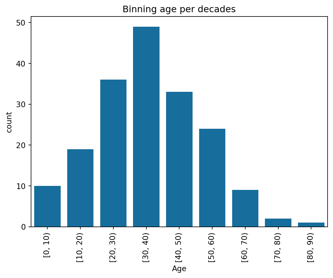
References