SciPy

Disclaimer: this course is adapted from the notebooks by

Introduction

SciPy is a scientific library that builds upon NumPy. Among others, SciPy deals with:

Integration (scipy.integrate)
Optimization (scipy.optimize)
Interpolation (scipy.interpolate)
Fourier Transform (scipy.fftpack)
Signal Processing (scipy.signal)
Linear Algebra (scipy.linalg)
Sparse matrices (scipy.sparse)
Statistics (scipy.stats)
Image processing (scipy.ndimage)
IO (input/output) (scipy.io)

%matplotlib inline
from scipy import linalg
import numpy as np
import matplotlib.pyplot as plt

References:

Matplotlib Animations / JavaScript Widgets by Louis Tiao

Animation with `plotly`

matplotlib works fine for advanced tuning, but is harder for simple tasks. So just try plotly for basic animations:

import plotly.express as px
from plotly.offline import plot

df = px.data.gapminder()
fig = px.scatter(
    df,
    x="gdpPercap",
    y="lifeExp",
    animation_frame="year",
    animation_group="country",
    size="pop",
    color="continent",
    hover_name="country",
    log_x=True,
    size_max=55,
    range_x=[100, 100000],
    range_y=[25, 90],
)
fig.show("notebook")

Linear algebra

scipy for linear algebra : use linalg. It includes functions for solving linear systems, eigenvalues decomposition, SVD, Gaussian elimination (LU, Cholesky), etc.

References:

Scipy documentation

Solving linear systems:

Find x such that: A x = b for specified matrix A and vector b.

A = np.array([[1, 0, 3], [4, 5, 12], [7, 8, 9]], dtype=float)
b = np.array([[1, 2, 3]], dtype=np.float64).T

print(A, b)

x = linalg.solve(A, b)
print(x, x.shape, b.shape)

[[ 1.  0.  3.]
 [ 4.  5. 12.]
 [ 7.  8.  9.]] [[1.]
 [2.]
 [3.]]
[[ 0.8       ]
 [-0.4       ]
 [ 0.06666667]] (3, 1) (3, 1)

Check the result at a given precision (different from ==)

np.allclose(A @ x, b, atol=1e-14, rtol=1e-15)

True

Remark: NEVER (or you should really know why) invert a matrix. ALWAYS solve linear systems instead!

Eigenvalues/ Eigenvectors

A v_n = \lambda_n v_n with v_n the n-th eigen vector and \lambda_n the n-th eigen value. The associated python functions are eigvals and eig:

A = np.random.randn(3, 3)
A = A + A.T
evals, evecs = linalg.eig(A)
print(evals, "\n ------\n", evecs)

np.allclose(A, evecs @ np.diag(evals) @ evecs.T)

[-1.72255542+0.j  1.21145677+0.j -0.08764969+0.j] 
 ------
 [[ 0.22923591 -0.8827723   0.41007799]
 [-0.91820064 -0.05629426  0.39209506]
 [ 0.32304562  0.46641614  0.82346676]]

True

EXERCISE: Eigenvalues/Eigenvectors

Verify numerically that the outputs from linalg.eig are indeed approximately eigenvalues and eigenvectors of matrix A above.

Hint: use Scipy documentation on allclose

Symmetric matrices

If A is symmetric you should use eigvalsh (H for Hermitian) instead: This is more robust and leverages the structures (you know they are real!)

Matrix operations

linalg.trace(A) # trace
linalg.det(A) # determinant
linalg.inv(A) # Inverse, consider NEVER using it though :)

Norms

print(linalg.norm(A, ord="fro"))  # fro for Frobenius
print((np.sum(A ** 2)) ** 0.5)
print(linalg.norm(A, ord=2))
print((linalg.eigvalsh(A.T @ A) ** 0.5))
print(linalg.norm(A, ord=np.inf))

2.107725588940538
2.1077255889405384
1.7225554211232876
[0.08764969 1.21145677 1.72255542]
2.3214277514508685

EXERCISE: Norms computation

Check numerically what the instruction linalg.norm(A, ord=np.inf) is computing. Double check with the help and a numerical test.

A = np.random.randn(3, 3)
print(linalg.norm(A, ord=np.inf))

2.336494930721582

Random generation, distributions, etc.

References:

Good practices with numpy random number generators by Albert Thomas
Numpy documentation on RandomState
Random Widgets, by Joseph Salmon: Visualization of various popular distributions.

seed = 12345
rng = np.random.default_rng(seed)  # can be called without a seed
rng.random()

0.22733602246716966

Optimization

Goal: find functions minima or maxima

References:

Scipy Lectures on mathematical optimization.

from scipy import optimize

Finding (local!) minima

def f(x):
    return 4 * x ** 3 + (x - 2) ** 2 + x ** 4


def mf(x):
    return -(4 * x ** 3 + (x - 2) ** 2 + x ** 4)


xs = np.linspace(-5, 3, 100)
plt.figure()
plt.plot(xs, f(xs))
plt.show()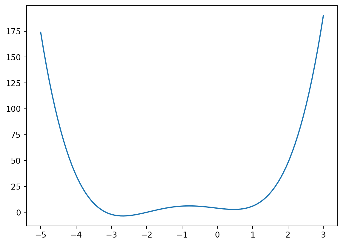

Default solver for minimization/maximization: fmin_bfgs (see Wikipedia on BFGS)

x_min = optimize.fmin_bfgs(f, x0=-4)
x_max = optimize.fmin_bfgs(mf, x0=-2)
x_min2 = optimize.fmin_bfgs(f, x0=2)


plt.figure()
plt.plot(xs, f(xs))
plt.plot(x_min, f(x_min), "o", markersize=10, color="orange")
plt.plot(x_min2, f(x_min2), "o", markersize=10, color="red")
plt.plot(x_max, f(x_max), "|", markersize=20)
plt.show()

Optimization terminated successfully.
         Current function value: -3.506641
         Iterations: 7
         Function evaluations: 16
         Gradient evaluations: 8
Optimization terminated successfully.
         Current function value: -6.201654
         Iterations: 5
         Function evaluations: 12
         Gradient evaluations: 6
Optimization terminated successfully.
         Current function value: 2.804988
         Iterations: 7
         Function evaluations: 16
         Gradient evaluations: 8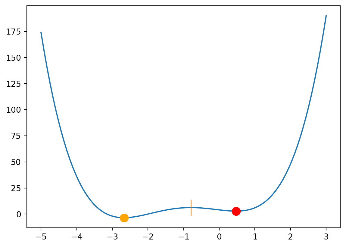

EXERCISE: Basin of attraction

Draw the points on the curves with two different colors :

orange: for the points leading to find the left local minima
red: for the points leading to the right local minima.

Find the zeros of a function

Find x such that f(x) = 0, with fsolve.

omega_c = 3.0

def f(omega):
    return np.tan(2 * np.pi * omega) - omega_c / omega


x = np.linspace(1e-8, 3.2, 1000)
y = f(x)

# Remove vertical lines when the function flips signs
mask = np.where(np.abs(y) > 50)
x[mask] = y[mask] = np.nan
plt.plot(x, y)
plt.plot([0, 3.3], [0, 0], "k")
plt.ylim(-5, 5)

optimize.fsolve(f, 0.72)
optimize.fsolve(f, 1.1)
optimize.fsolve(f, np.linspace(0.001, 3, 20))
np.unique(np.round(optimize.fsolve(f, np.linspace(0.2, 3, 20)), 3))

my_zeros = (
    np.unique((optimize.fsolve(f, np.linspace(0.2, 3, 20)) * 1000).astype(int)) / 1000.0
)
plt.figure()
plt.plot(x, y, label="$f$")
plt.plot([0, 3.3], [0, 0], "k")
plt.plot(my_zeros, np.zeros(my_zeros.shape), "o", label="$x : f(x)=0$")
plt.legend()
plt.show()

Parameters estimation

from scipy.optimize import curve_fit


def f(x, a, b, c):
    """f(x) = a exp(-bx) + c."""
    return a * np.exp(-b * x) + c


x = np.linspace(0, 4, 50)
y = f(x, 2.5, 1.3, 0.5)  # true signal
yn = y + 0.2 * np.random.randn(len(x))  # noisy added

plt.figure()
plt.plot(x, yn, ".")
plt.plot(x, y, "k", label="$f$")
plt.legend()
plt.show()

(a, b, c), _ = curve_fit(f, x, yn)
print(a,"\n", b,"\n", c)

2.5317783963846265 
 1.0129483612063013 
 0.4118272634943516

Displaying

plt.figure()
plt.plot(x, yn, ".", label="data")
plt.plot(x, y, "k", label="True $f$")
plt.plot(x, f(x, a, b, c), "--k", label="Estimated $\hat{f}$")
plt.legend()
plt.show()

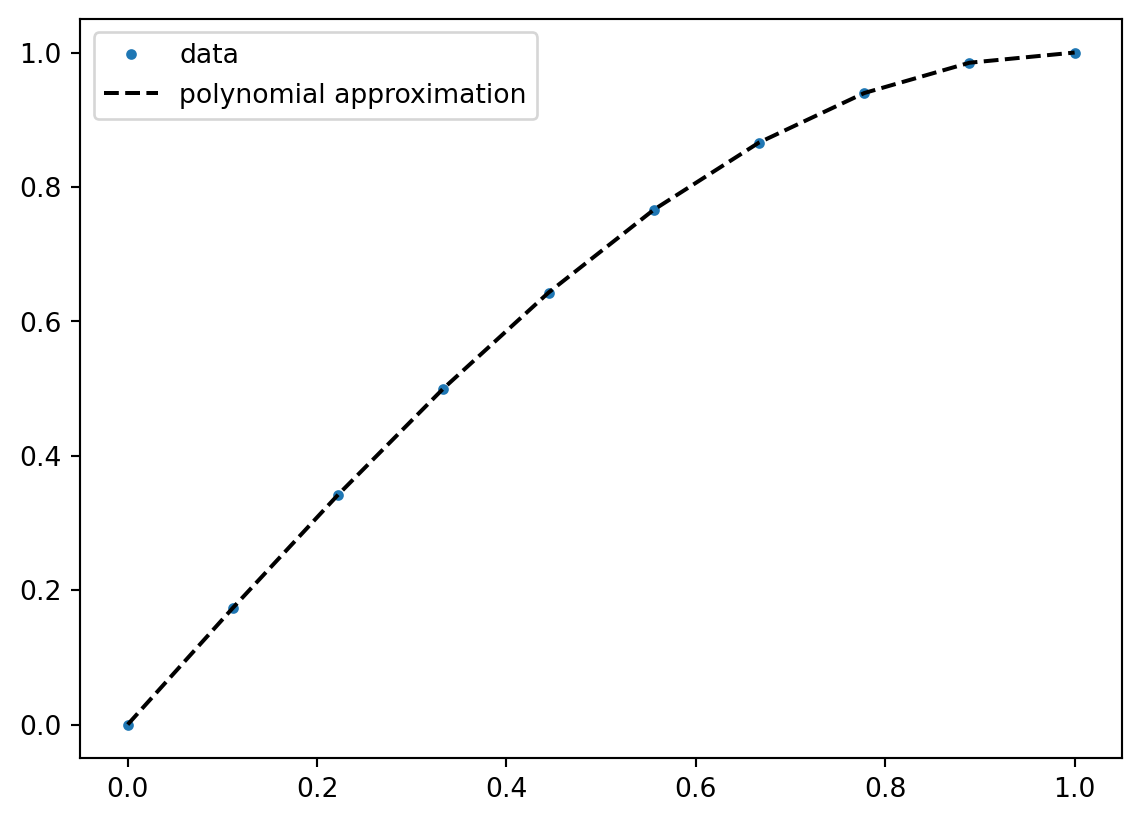
For polynomial fitting, one can directly use numpy functionsL

x = np.linspace(0, 1, 10)
y = np.sin(x * np.pi / 2.0)
line = np.polyfit(x, y, deg=10)
plt.figure()
plt.plot(x, y, ".", label="data")
plt.plot(x, np.polyval(line, x), "k--", label="polynomial approximation")
plt.legend()
plt.show()

/home/jsalmon/anaconda3/envs/peerannot/lib/python3.10/site-packages/IPython/core/interactiveshell.py:3548: RankWarning:

Polyfit may be poorly conditioned

Interpolation

from scipy.interpolate import interp1d, CubicSpline


def f(x):
    return np.sin(x)


n = np.arange(0, 10)
x = np.linspace(0, 9, 100)

y_meas = f(n) + 0.1 * np.random.randn(len(n))  # add noise
y_real = f(x)

linear_interpolation = interp1d(n, y_meas)
y_interp1 = linear_interpolation(x)

cubic_interpolation = CubicSpline(n, y_meas)
y_interp2 = cubic_interpolation(x)


plt.figure()
plt.plot(n, y_meas, "bs", label="noisy data")
plt.plot(x, y_real, "k", lw=2, label="true function")
plt.plot(x, y_interp1, "r", label="linear interp")
plt.plot(x, y_interp2, "g", label="CubicSpline interp")
plt.legend(loc=3)
plt.show()

Images

RGB decomposition

First, discuss the color decomposition in RGB. The RGB color model is an additive color model[1] in which the red, green and blue primary colors of light are added together in various ways to reproduce a broad array of colors. Hence, each channel (R, G or B) represents a grayscale image, usually coded on [0,1] or [0,255].

from scipy import ndimage, datasets

img = datasets.face()
print(type(img), img.dtype, img.ndim, img.shape)

print(2 ** 8)  # uint8-> code sur 256 niveau.

n_1, n_2, n_3 = img.shape
print(n_1, n_2, n_3)

# True image
plt.figure()
plt.imshow(img)
plt.axis("off")
plt.show()

<class 'numpy.ndarray'> uint8 3 (768, 1024, 3)
256
768 1024 3

fig, ax = plt.subplots(3, 2)
fig.set_size_inches(7, 4.5)
n_1, n_2, n_3 = img.shape

# add subplot titles
ax[0, 0].set_title("Red channel")
ax[0, 0].imshow(img[:, :, 0], cmap=plt.cm.Reds)
ax[0, 1].set_title("Pixel values histogram (red channel)")
ax[0, 1].hist(img[:, :, 0].reshape(n_1 * n_2), np.arange(0, 256))

ax[1, 0].set_title("Green channel")
ax[1, 0].imshow(img[:, :, 1], cmap=plt.cm.Greens)
ax[1, 1].set_title("Pixel values histogram (green channel)")
ax[1, 1].hist(img[:, :, 1].reshape(n_1 * n_2), np.arange(0, 256))

ax[2, 0].set_title("Blue channel")
ax[2, 0].imshow(img[:, :, 2], cmap=plt.cm.Blues)
ax[2, 1].set_title("Pixel values histogram (blue channel)")
ax[2, 1].hist(img[:, :, 2].reshape(n_1 * n_2), np.arange(0, 256))

plt.tight_layout()

print(img.flags)  # cannot edit...
img_compressed = img.copy()
img_compressed.setflags(write=1)
print(img_compressed.flags)  # can edit now


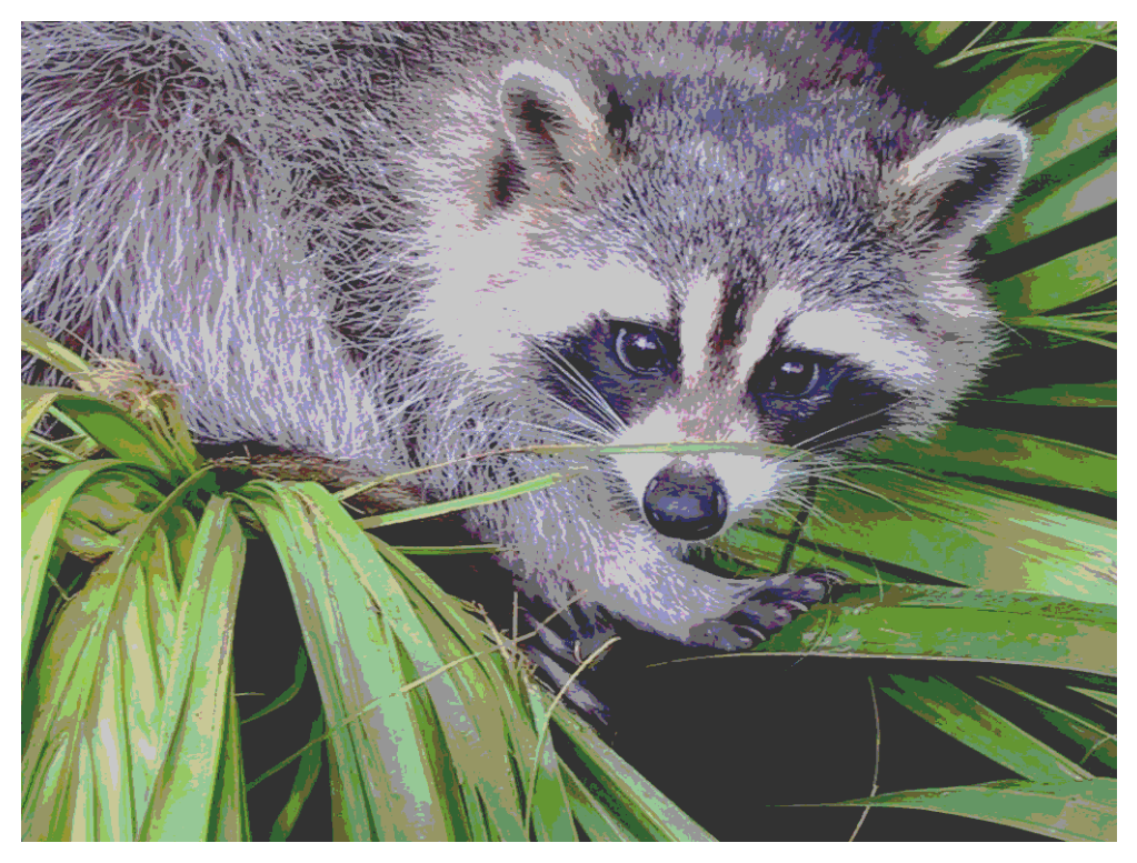
img_compressed[img_compressed < 70] = 50
img_compressed[(img_compressed >= 70) & (img_compressed < 110)] = 100
img_compressed[(img_compressed >= 110) & (img_compressed < 180)] = 150
img_compressed[(img_compressed >= 180)] = 200
plt.figure()
plt.imshow(img_compressed, cmap=plt.cm.gray)
plt.axis("off")
plt.show()

  C_CONTIGUOUS : True
  F_CONTIGUOUS : False
  OWNDATA : False
  WRITEABLE : False
  ALIGNED : True
  WRITEBACKIFCOPY : False

  C_CONTIGUOUS : True
  F_CONTIGUOUS : False
  OWNDATA : True
  WRITEABLE : True
  ALIGNED : True
  WRITEBACKIFCOPY : False

Convert a color image in grayscale

plt.figure()
plt.imshow(np.mean(img, axis=2), cmap=plt.cm.gray)
plt.show()

Changing colors in an image

import pooch
import os

url = "https://upload.wikimedia.org/wikipedia/en/thumb/0/05/Flag_of_Brazil.svg/486px-Flag_of_Brazil.svg.png"
name_img =pooch.retrieve(url, known_hash=None)

img = (255 * plt.imread(name_img)).astype(int)
img = img.copy()
plt.figure()
plt.imshow(img)

fig, ax = plt.subplots(3, 2)
fig.set_size_inches(7, 4.5)
n_1, n_2, n_3 = img.shape

ax[0, 0].imshow(img[:, :, 0], cmap=plt.cm.Reds)
ax[0, 0].set_title("Red channel")
ax[0, 1].hist(img[:, :, 0].reshape(n_1 * n_2), np.arange(0, 256), density=True)
ax[0, 1].set_title("Pixel values histogram (red channel)")

ax[1, 0].imshow(img[:, :, 1], cmap=plt.cm.Greens)
ax[1, 0].set_title("Green channel")
ax[1, 1].hist(img[:, :, 1].reshape(n_1 * n_2), np.arange(0, 256), density=True)
ax[1, 1].set_title("Pixel values histogram (green channel)")

ax[2, 0].imshow(img[:, :, 2], cmap=plt.cm.Blues)
ax[2, 0].set_title("Blue channel")
ax[2, 1].hist(img[:, :, 2].reshape(n_1 * n_2), np.arange(0, 256), density=True)
ax[2, 1].set_title("Pixel values histogram (Blue channel)")
plt.tight_layout()

EXERCISE: Make the Brazilian italianer

Create a version of the Brazilian flag as follows:

RGBA

RGBA stands for red (R), green (G), blue (B) and alpha (A). Alpha indicates how the transparency allows an image to be combined over others using alpha compositing, with transparent areas.

Hexadecimal decomposition

Often, colors are represented not with an RGB triplet, say (255, 0, 0), but with a hexadecimal code (say #FF0000). To get a hexadecimal decomposition, transform each 8-bit RGB channel (i.e., 2^8=256) into a 2-digit hexadecimal number (i.e., 16^2=256). This requires letters for representing 10: A, 11: B,\dots, 15: FF (see https://www.rgbtohex.net/ for an online converter)

CMYK decomposition

This is rather a subtractive color model, where the primary colors are cyan (C), magenta (M), yellow (Y), and black (B). For a good source to go from RGB to CMYK (and back), see https://fr.wikipedia.org/wiki/Quadrichromie.

HSL (hue, saturation, lightness)

XXX TODO.

Here, you can find a simple online converter for all popular color models: https://www.myfixguide.com/color-converter/.

Image files formats

Bitmap formats: - PNG (raw, uncompressed format, opens with Gimp) - JPG (compressed format) - GIF (compressed, animated format)

Vector formats: - PDF (recommended for your documents) - SVG (easily modifiable with Inkscape) - EPS - etc.

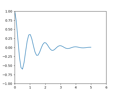
x1 = np.linspace(0.0, 5.0, num=50)
x2 = np.linspace(0.0, 2.0, num=50)
y1 = np.cos(2 * np.pi * x1) * np.exp(-x1)
y2 = np.cos(2 * np.pi * x2)

fig1 = plt.figure(figsize=(5, 4))
plt.plot(x1, y1)
plt.xlim(0, 6)
plt.ylim(-1, 1)

Then, we can save the figure in various formats:

fig1.savefig("ma_figure_pas_belle.png", format='png', dpi=90)
fig1.savefig("ma_figure_plus_belle.svg",format='svg', dpi=90)

Now that the images have been saved, we can visualize the difference between the PNG and SVG formats.

PNG (zoom on hover):

SVG (zoom on hover):

Note

Some additional effects to produce the above zoom-on-hover effect can be found here: https://www.notuxedo.com/effet-de-zoom-image-css/

References:

Introduction to geopandas
Course on images/slides by Joseph Salmon
Official SciPy web page
SciPy User Guide
Scipy lectures
The SciPy source code

Introduction

Animation with plotly

Linear algebra

Solving linear systems:

Eigenvalues/ Eigenvectors

Symmetric matrices

Matrix operations

Norms

Random generation, distributions, etc.

Optimization

Finding (local!) minima

Find the zeros of a function

Parameters estimation

Interpolation

Images

RGB decomposition

Convert a color image in grayscale

Changing colors in an image

RGBA

Hexadecimal decomposition

CMYK decomposition

HSL (hue, saturation, lightness)

Image files formats

Animation with `plotly`